The popular crystallographic rebuilding program Coot also has the capability of using probe dots as an aid in model changes. In this part, you will use Coot to rebuild Thr 32 in 1SBP, a sulfate-binding protein at 1.7Å resolution.
Prepare the set-up for using Coot with all-atom contacts
Check that two programs from our lab are installed and on your PATH -- Reduce - to add hydrogens to proteins, nucleic acids, and ligands, and Probe - to generate the contact dots. From the command line of a terminal type:
shell>which reduce and then, shell>which probe,
to get a report that these programs are in your PATH.
For the record, the .coot contents are: (define *probe-command* "/full/path/to/probe")
(define *reduce-command* "/full/path/to/reduce")
(set-find-hydrogen-torsion 1)
(set-do-probe-dots-on-rotamers-and-chis 1)
(set-do-probe-dots-post-refine 1)
(set-rotamer-lowest-probability 0.5)
Get the Coot set-up file, ~/.coot needed for this exercise in your home directory, type:
shell>cd shell>cp ~dcr/.coot .
This sets up to do Probe dots when you rebuild or refine, and to use a wider range of sidechain rotamers.
Fire-up Coot and read in the model and map
Type the command to start-up Coot:
shell> coot
Adjust the Coot windows to your preferred work habits.
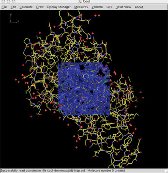
Read in the coordinate file and maps from the Uppsala Electron Density server (EDS), using the menu item: File > Get PDB & Map using EDS ...
Activating this menu item will bring up a box requesting the "PDB Accession Code". Click in the field, type "1sbp", and press return. This will lead to numerous informational messages in the Coot terminal and eventually, hopefully the model and a map section will be drawn in the Coot graphics window.
Check-out the model vs all-atom contact dots and electron-density map
In the previous session on MolProbity, one potential area of interest for 1sbp was the threonine residue 32. Having two sets of bad-overlap contact dots, a high Cβ deviation, and a bad rotamer score, this area is "yelling for help". In this section, we will use all-atom contact analysis to help us rebuild that area/residue.
Use the Coot To Do list generated by MolProbity (1sbpH-multi-coot.scm) that you downloaded. It can be read into Coot via the menu item: Calculate > Run Script...
On the to-do list window, find the 4th group (called "321 HOH") and click on one of the buttons for Thr 32.
Use the built-in functionality of Coot to display all-atom contacts.
Use the menu item: Validate > Probe clashes > 0 pdb1sbp.ent to calculate and show all the contact dots.
After you select the Probe clashes menu item, Reduce will add hydrogens to the model #0 (or whichever you selected in the submenu), Probe will add contact dots to the reduced model and eventually the dots will show in the Coot graphics window. Extra windows come up to let you turn the classes of dots on or off, etc.
Note the red clash spikes between the Thr methyl and a backbone NH, and the relative density and difference density of the O vs C sidechain branches. Look down the Cb-Ca bond to see that chi1 is eclipsed and the Og-Cb-Cg bond angle is much wider than tetrahedral.
Turn off display of molecule 0, the original 1sbp model.
Coot creates a new molecule (#3) for the protonated-1sbp. Turn off the display of the original using the Display Manager. This will simplify display and picking in future steps.
See if another rotamer helps
In the diagnosis/MolProbity session on 1sbp, we saw that Thr 32 is a rotamer outlier. So, a good place to start is to see if there is a standard rotamer that can be substituted that is consistent with the map and also relieves the contact dots overlap error signal. Coot has an internal rotamer library that can be used for this test.
Invoke the rotamer library via the Model/Fit/Refine floating menu. This floating rainbow-colored menu is displayed by first doing the menu sequence: Calculate > Model/Fit/Refine...
Then, click the Rotamers... item in this floating menu.
After clicking the Rotamers... item, Coot will prompt you (in the terminal window) to "Click on an atom in a residue for which you wish to see rotamers". Doing so in the graphics window will lead to display of an alternate rotamer (colored white for our instance) and a "Select Rotamer" dialog box. The box contains information about each rotamer for that residue in the library.
Alternate rotamers can be cycled through by either pressing the "." (period) or "," (comma) keys while in graphics window focus; or by clicking on the rotamer list presented in the "Select Rotamer" dialog box.
Unfortunately, probe dots are not updated interactively as one flips through the rotamer palette. Rather, to see the contact dots for the rotamer, you must "Accept" (click on that button in the "Select Rotamer" dialog box) and then the dots will be updated. Not much of a problem for 3-state Thr, as you can try each rotamer that way, and if not finding any of interest, recover molecule 0.
Evaluate the available threonine rotamers versus the map and contact dots. Select one if you think you are better off than with the current non-rotameric conformer. One of the three rotamers fits the density shape better than the present model (consider the positive difference-density), is a rotamer, and with some torsion-angle adjustments done below can eliminate the bad contacts (bad overlap) and increase the good contacts (hydrogen-bonding).
Improve the fit to map using real space refinement
After selecting a rotamer, we're left with a slightly poorer fit to the map. But contrariwise, the map is biased to the original model; relocation of the OG1 helps explain the positive difference density; the original CB placement yields a high Cβ difference; the map density for the OG1-CB-CG2 sidechain is linear, rather than lobed (cf. Thr 96) and there is a hint that this straight portion may be bent as with the proposed rotamer. With this accumulated evidence, its reasonable to think that refinement and a new map will lead to a better explanation of the data. Let's use the current map to improve the model's fit locally.
Select the Select Map... item from the Model/Fit/Refine floating menu. From the dialog-box choose the 2FoFc map to use for refinement.
Next choose the Real Space Refine Zone item. You will be prompted to set the refine zone by choosing two atoms. Select the same atom twice to refine only the threonine 32 residue. After "a miracle occurs" the proposed solution will be displayed (again in white for our instance). Decide whether to accept or reject. If you're a miracle worker, you may want to fiddle with the weightings discussed in Coot's help manual.
For the example being worked on for this write-up, rotamer selection and real space refinement has eliminated the pink spikes of the contact dots.
But we're not done yet ...
Twiddle with the fit using torsion angles
Rotating the threonine's side chain oxygen round not only uses the rotamer of highest frequency, it also creates a new hydrogen bond between the amide hydrogen of ASP 34 and the THR 32 OG. With rotation of the OG1-HG1 hydroxyl bond yet another H-bond can be created between this hydroxyl hydrogen and the carbonyl oxygen of TRP 28.
Activate the ability to change Chi Angles via selecting Edit Chi Angles from the (still) floating Model/Fit/Refine menu. You'll be asked to "Click on an atom in the residue that you want to edit" (e.g., the Cα).
You'll get a new dialog box popped up - drag it out of the way and forget about it until the end. Make all your adjustments while focussed in the Coot graphics window. The mouse mappings are confusing: CTRL-left-drag moves the view while left-drag moves the torsion angle. Choose the torsion angle by typing a number (1, 2 or 3 in this case) that corresponds to the list placement of the torsion in that pop-up we had you hide.
We want to change the CA-CB-OG1-HG1 torsion which is #2 in the list. So make sure you have graphics window focus, then type 2, then left drag to move the HG1. If you need to change the view, do a CTRL-LEFT-drag. Curse silently when you forget the CTRL toggle. Contact dots interactively update.
Commit to the change by selecting "Accept" in that hidden dialog box.
Congratulations, you've rebuilt a problem area.
At this point, write out the coordinates for optional use later. File > Save Coordinates does that.
This technique is now available to you whenever fitting or validating. It is most valuable, and easiest to apply, when done during the refinement and rebuilding process rather than waiting until the end. Use it whenever you are trying to make a difficult decision between alternatives, run the overall validation (as in the first part of this exercise) occasionally to find problems you might have overlooked, and be sure to check one last time before depositing coordinates.

 Type the command to start-up Coot:
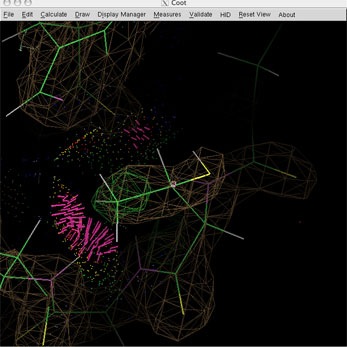 Use the Coot To Do list generated by MolProbity (1sbpH-multi-coot.scm) that you downloaded. It can be read into Coot via the menu item: Calculate > Run Script...
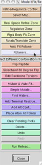 Invoke the rotamer library via the Model/Fit/Refine floating menu. This floating rainbow-colored menu is displayed by first doing the menu sequence: Calculate > Model/Fit/Refine...