Part 1: MolProbity Analysis

Analyze 1BKR on the website.

Fire-up MolProbity and read in the model

1. MolProbity is a web service hosted on the WWW by the Richardson Lab at Duke University. MolProbity's Main Page can be accessed directly via the server address: http://molprobity.biochem.duke.edu/ and via the Richardson Lab website http://kinemage.biochem.duke.edu/.
2. There is no set-up required for MolProbity - it will run in most browser. Chrome is being used at the example here.
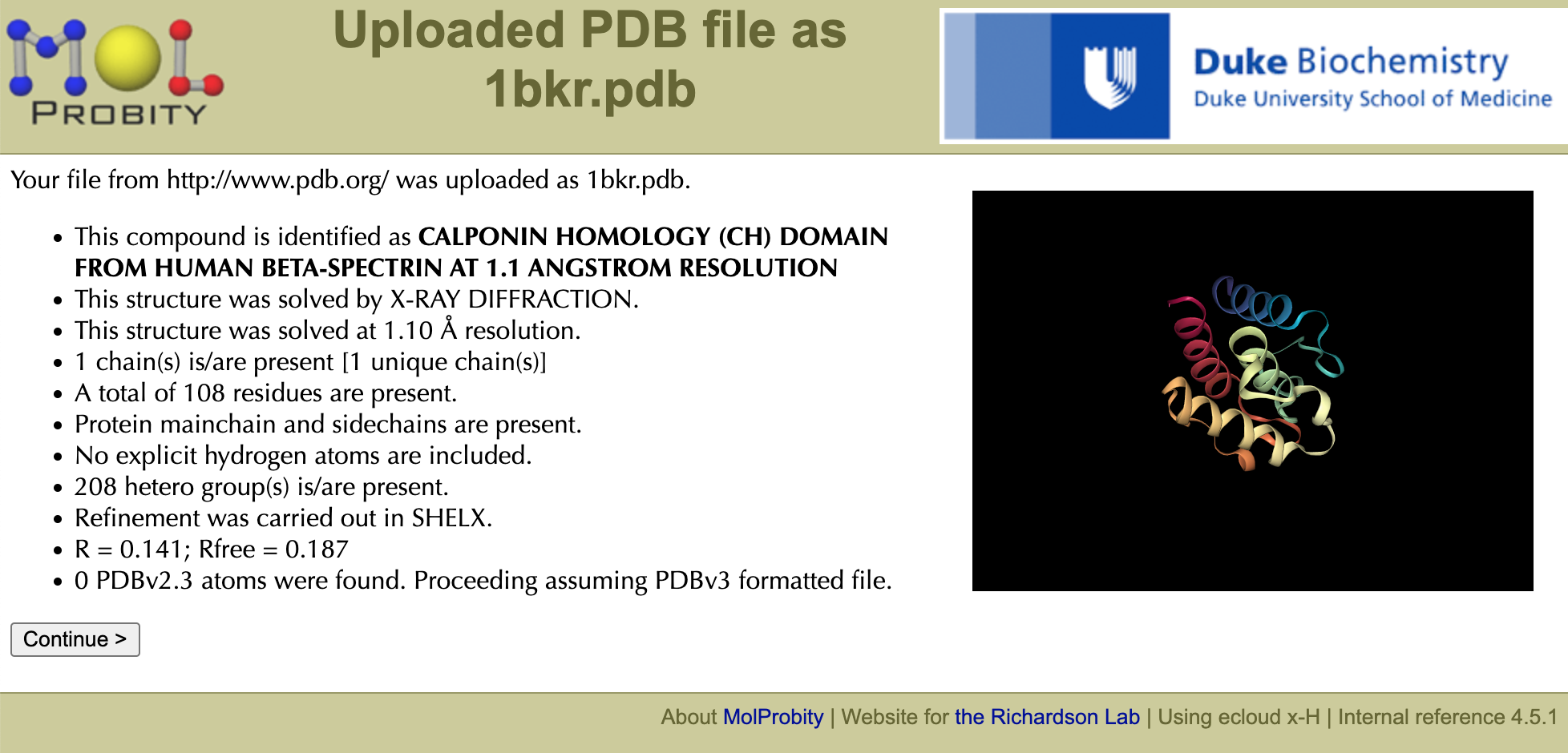
3. Enter "1bkr" in the field for choosing a PDB/NDB code and click "Fetch >". Note molecule identity (CH domain), resolution (1.1Å), number of chains/residues (1/108), crystallographic details, etc. in the resulting info panel. A small interactive thumbnail using the NGL Viewer Javascript program is provided, which lets you see if you mistyped the PDB code (e.g. 0 vs o) or if there are more molecules in the asymmetric unit than you wanted, etc. Click the "Continue >" button to continue to the MolProbity main page.
   

Add hydrogens & evaluate Asn/Gln/His flips

Notice that two additional panes are now present on the MolProbity Main Page. Options available while running MolProbity are context-sensitive. Before loading a coordinate file, you had two panes - "File Upload/Retrieval" and MolProbity information; after loading "1bkr", you now also have a "Suggested Tools" pane to work on the indicated coordinate file and a "Recently Generated Results" pane to manage the files in your work area about the original two.
The tools available in the "Suggested Tools" pane are also context sensitive. We will use the "Add hydrogens" option next; but one could instead first edit the PDB file here, if for instance, there were multiple identical chains in the asymmetric unit and you wanted to focus on just one.

1. Choose the "Add hydrogens" function, and accept the defaults on the next dialog-page: "Start adding H >", to run Reduce with Asn/Gln/His flips and electron-cloud x-H distances.
2. All suggested flips are for His (no Asn or Gln) and seem like clear wins from the scores. You will later download the 1bkrFH-fliphis.kin file ("his", not "nq") to study offline.
3. You have the choice of rejecting a flip if you don't agree with it. [That's rare, but can happen, especially if you have access to extra information. For example, if a flip state is completely unambiguous in one crystal form (e.g. with ligand bound), then "some evidence" is probably not enough to justify fitting it differently in another crystal form.] These 4 His flips in 1bkr should very clearly all be accepted, so just click the "Regenerate H,..." button, which moves you on to a flip-report page. Note the information presented on this report and then "Continue >" to the MolProbity Main Page.

Analyze all-atom contacts and geometry

The Suggested Tools pane now includes the "Analyze all-atom contacts and geometry" tool as you are now working on a coordinate file with hydrogens. Select this tool, and then "Run..." with the default settings. NOTE: If your file is extraordinarily large, the default option "Create html version of multichart" is turned off. The run initiates calculation of the set of analyses requested. However, note that analysis steps are checked off as they are completed and some present links to results immediately viewable. So, if you tire of spinning-SOD, you can look at results before all of the requested set is complete. Otherwise, you'll see next the "Analysis output: all-atom contacts and geometry for 1bkrFH.pdb" report. From this page you can see the summary statistics or choose to view any of the requested model quality assessments. Discussed below are the items requested for 1bkrFH.

Summary Statistics & Multi-criterion chart

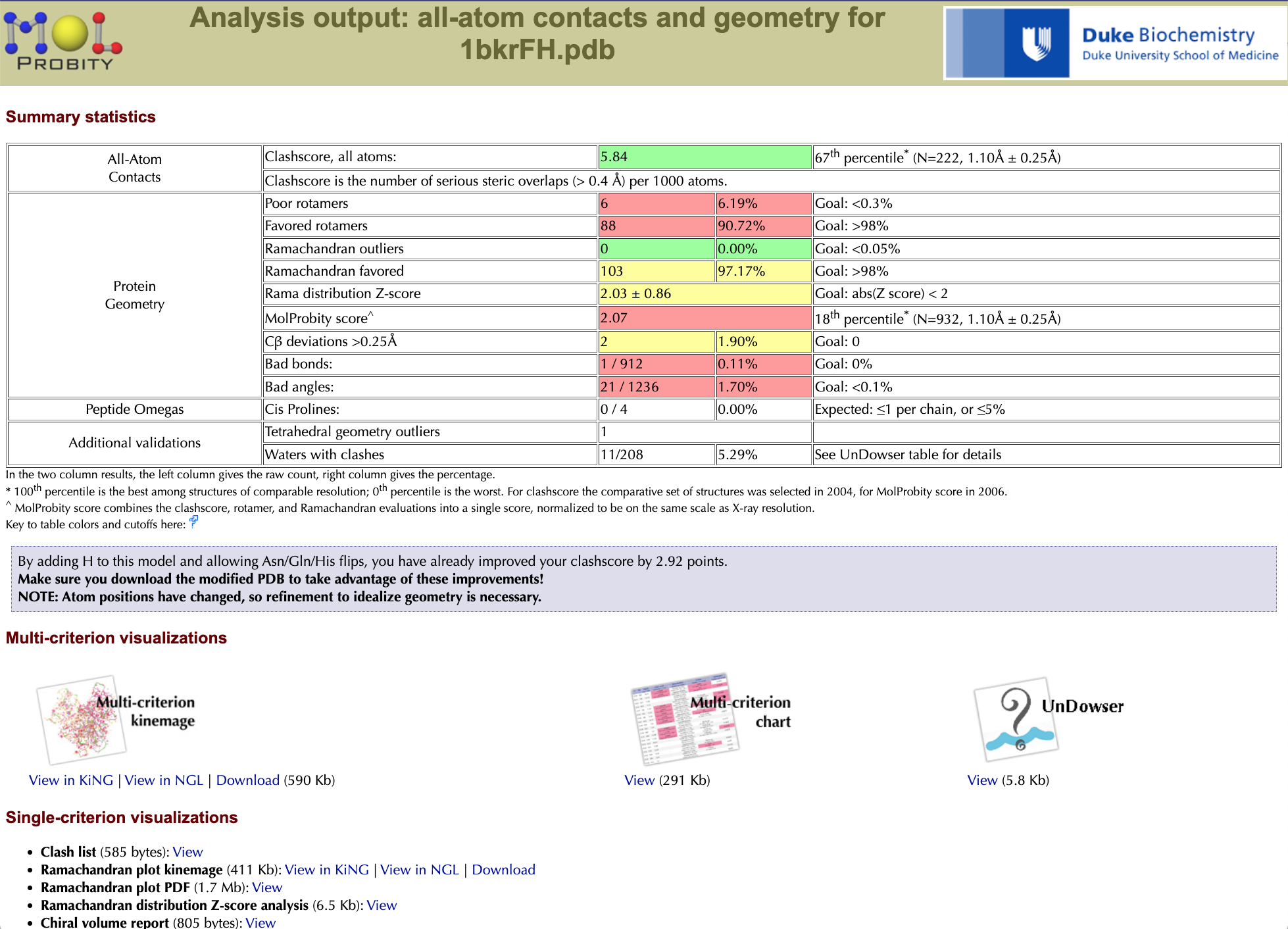The summary statistics for 1bkr show excellent Ramachandran values, but mediocre sterics and poor sidechain rotamers for this resolution range. No backbone bond lengths or angles deviate >4σ, but there are two Cβ deviations (see below) >0.25 Angstrom. The important thing, though, is not the overall scores, but the specific good or bad local regions that produce them. Click on "View" under the "Multi-criterion chart" to open a residue-by-residue validation table in a new browser tab/window. It comes up ordered by residue number. Scroll down, to see that both N- and C-terminal residues have problems (very common, even at atomic resolution). A click on the title of any column sorts the list by its values: try "Rotamer", to put the most suspect sidechains first, and note that other pink outliers are also enriched. [A misfitting typically shows up on more than one validation criterion.] Both chain termini (res 2 & 109) and the two Thr's are outliers in 2 or 3 columns. In a 100-res protein it would be plausible to have one rotamer <1% score that was valid; however, in 1bkr all 6 are in fact wrong. Click on "Close this (chart) window" or close the tab to go back to the main summary window.

Online interactive viewing

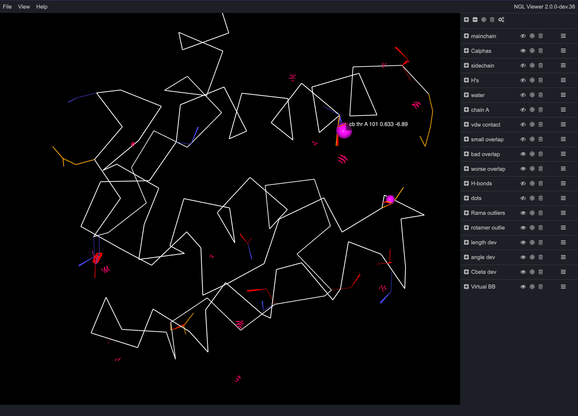Under Multi-criterion visualizations, under Multi-criterion kinemage, click on the "View in NGL" link. This opens a new browser window with an 3D interactive view of the protein with a variety of markup to indicate areas of the structure with validation issues. Hovering over the different points in the interface will show a popup containing the information for that particular atom/residue/issue. Different groups can be turned on or off by clicking on the small eye icon next to the names of the groups. Note that viewing kinemage in NGL has limited functionality compared to viewing in KiNG, so for more in depth analysis and rebuilding, later we will be downloading the kinemage file for use in the standalone version of KiNG.

Download files for use offline below and in Part 2

1. Hit the "Continue" button at the bottom to go back to the main page. Scroll down to the file download section and then expand "coordinates" (by clicking the little triangle). Find the pdb file WITH the new H atoms: 1bkrFH.pdb, and download it (using the "download" link on the right side) to your working directory for this practical (best to right-click and "save link as"). Now expand "kinemages" and download 1bkrFH-multi.kin.gz and 1bkrFH-fliphis.kin. These will let you explore the content and logic of NQH flips and multi-kins shortly in the next section. Log out (on left side navigation panel), and "destroy" all files (Note in file names: F for Flipped, H for Hydrogens added).
2. Go to the RCSB Protein Data Bank website (https://www.rcsb.org/) and search for 1bkr using the search bar. On that summary page, note the quality sliders for 1bkr. Under the "Download files" dropdown menu on the 1bkr page, download the 2mFo-Dfc and mFo-Dfc dsn6-format electron density maps, then exit the browser. [Some of these files are compressed as *.gz, but you won't need to unzip them.] Now you have the files to continue working off-line with KiNG to rebuild selected residues in Part 2.

Examining MolProbity results offline

Go to the KiNG Quick-start page for a quick primer on basic usage of KiNG.

Histidine flips and protonation

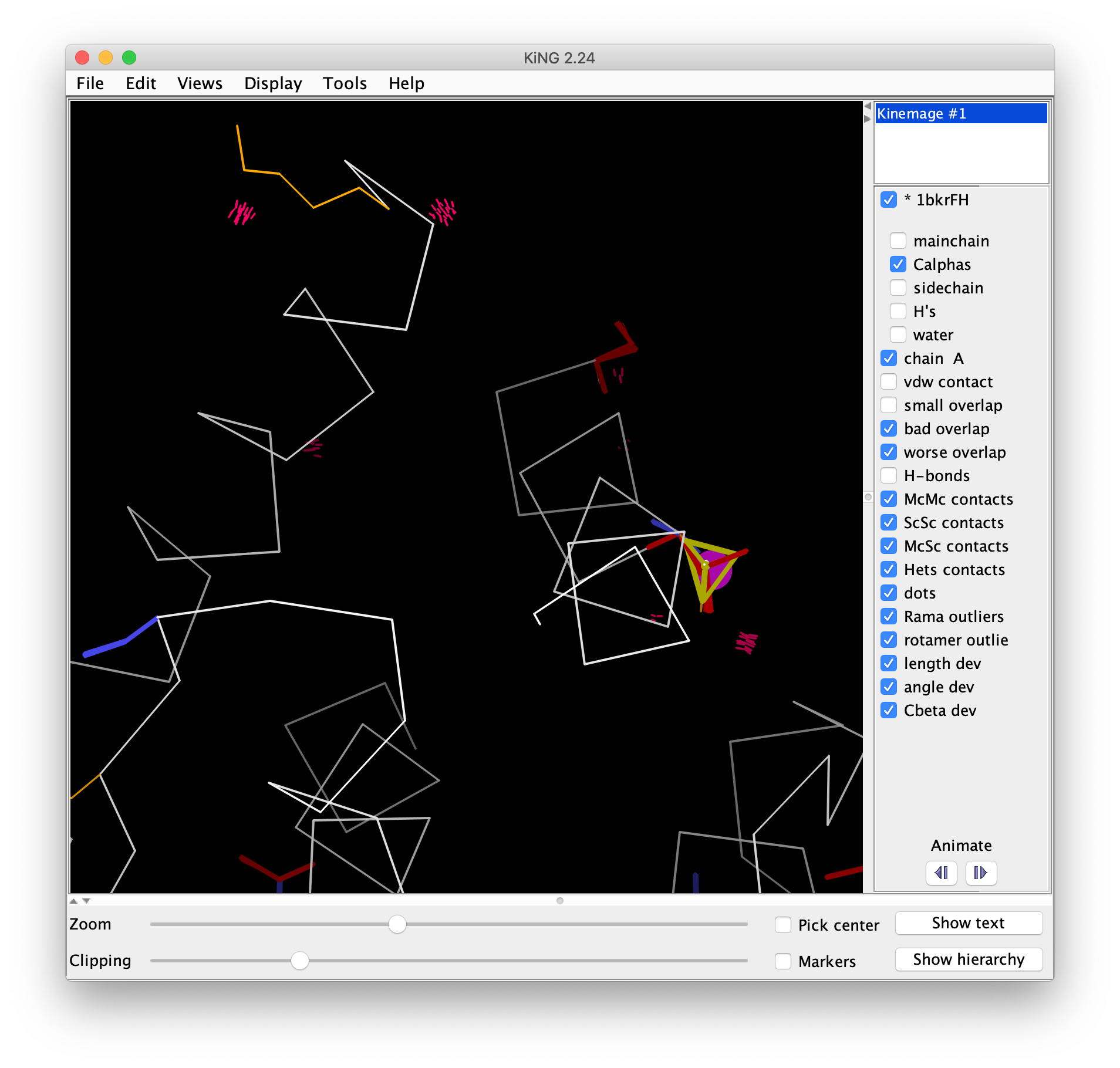
In your terminal, change to your your working directory, type “phenix.king”, then open 1bkrFH-fliphis.kin. The KiNG "Views" pulldown menu has an entry for each His, with * marking those flipped by Reduce; look at each * view. H25, H73, and H104 are clear and simple; rotate the viewpoint to see the H-bond partner(s), and to compare the two flip states use the "a" key or the Animate arrows in the lower right side panel. [The preferred state of the side chain is labeled “reduce” and colored green].

His 73, as shown definitively by contacts, does indeed need to be flipped. Note that both orientations are protonated at the NE2 position, but in the flipped orientation, the ND1 atom could potentially also be protonated and donate to the nearby water. Such protonation difference doesn't affect R factors, but the change in charge would destroy an MD or docking calculation; one has to really examine this case to see if double protonation would be more reasonable. Upon closer examination, the water nearest ND1 H-bonds to Arg 45. Arg is charged and an obligate donor, so this water is not likely to favorably receive another donated H from the His. Hence, His 73 is probably accepting an H from the water, and thus would be singly protonated on its NE2. It is important to note that the program Reduce, which adds hydrogens and optimizes N/Q/H orientations in MolProbity, does not take the Arg 45 into account when determining protonation state, and if the inter-atomic distances were slightly different, could double-protonate His 73. This emphasizes that there is no substitute for a person really looking, evaluating, and possibly making further changes as a model is constructed.

The correct flip for His42 is blindingly obvious visually or by score differences in MolProbity, but is puzzling to assign unaided, with 3 potential H-bonding groups nearby (turn to put the His ring flat and find the 3). The preferred flip state makes 2 good H-bonds (try turning off the "vdw contact" and "small overlap" buttons, for a clearer view of the pale green lenses of H-bonding dots). Measure each N to O distance (just pick the 2 atoms in succession, click on the "Markers" button near the bottom right of the KiNG window to help track your picks). Animate to the other flip state. The distance from the His42 ND1 to the Ile49 carbonyl O is too far (measure it) for anything but a very weak H-bond, while both ring CH's produce red clashes.

To confirm this flip in the electron density, drag-and-drop the 2mFo-Dfc map file onto the open KiNG window or open the map file using "Tools" > "Structural biology" > "Electron density maps", and confirm that the file is dsn6/Omap format. Animate back to the conformation that was preferred by Reduce. The ring electron density is quite clean, with no evidence of disorder. In the map dialog, move the purple contour level up to 4.7σ, where you should see differences between peak levels for N vs C atoms that corroborate Reduce's flip choice (in spite of model bias from having refined it the other way around). In clean density, the distances between neighbor atoms are quite sensitive indicators of whether or not they form an H-bond. Once you have confirmed the flip, use "File" > "Close" to close the kinemage file.

Multi-criterion kinemage

Open 1bkrFH-multi.kin.gz in KiNG either by dragging the file onto the open KiNG window, or by using "File" > "Open file" to select the kinemage file. The multi-criterion kinemage shows the Cα backbone, with all-atom clashes as hotpink spikes, bad Cβ deviations as magenta balls, poor rotamers as gold sidechains, and chiral volume outliers with heavy yellow lines (Ramachandran outliers would be flagged by heavy green lines, and bad bond angles in blue or red). Again, the two Thr and the chain termini show up clearly as clusters of problems. Go to Lys 2 (either locate it visually and right click to center, or use "Find point" on the "Edit" menu) and turn on buttons for mainchain, sidechain, H's, and water rather than Cαs. Check B-factors (click on atom and read info line at bottom of graphics window) for some non-terminal nearby Cαs as controls, which should be around 10. Then try the sidechain atoms of Lys 2; the clash with Asp 6 is probably just a misplacement of the Lys sidechain. The Lys N clashes with a water (both relatively low B); this can be well fit as the 1-2 peptide to the missing residue 1 in helical conformation (the water becomes the carbonyl O); optionally you can confirm this later by looking at the 2Fo-Fc map. The Multi-criterion kinemage contains a wealth of information, which we will use in part 2 to make corrections. For now, you can close the kinemage file.

Analyze an AlphaFold model.

Download a model from an AlphaFold database


1. As a separate exercise, before rebuilding 1BKR, we will run MolProbity to validate an AlphaFold model. Go to https://alphafold.ebi.ac.uk/ in a browser. This is an online database of AlphaFold structure predictions for many proteins, including the proteomes of many model organisms and pathogens.
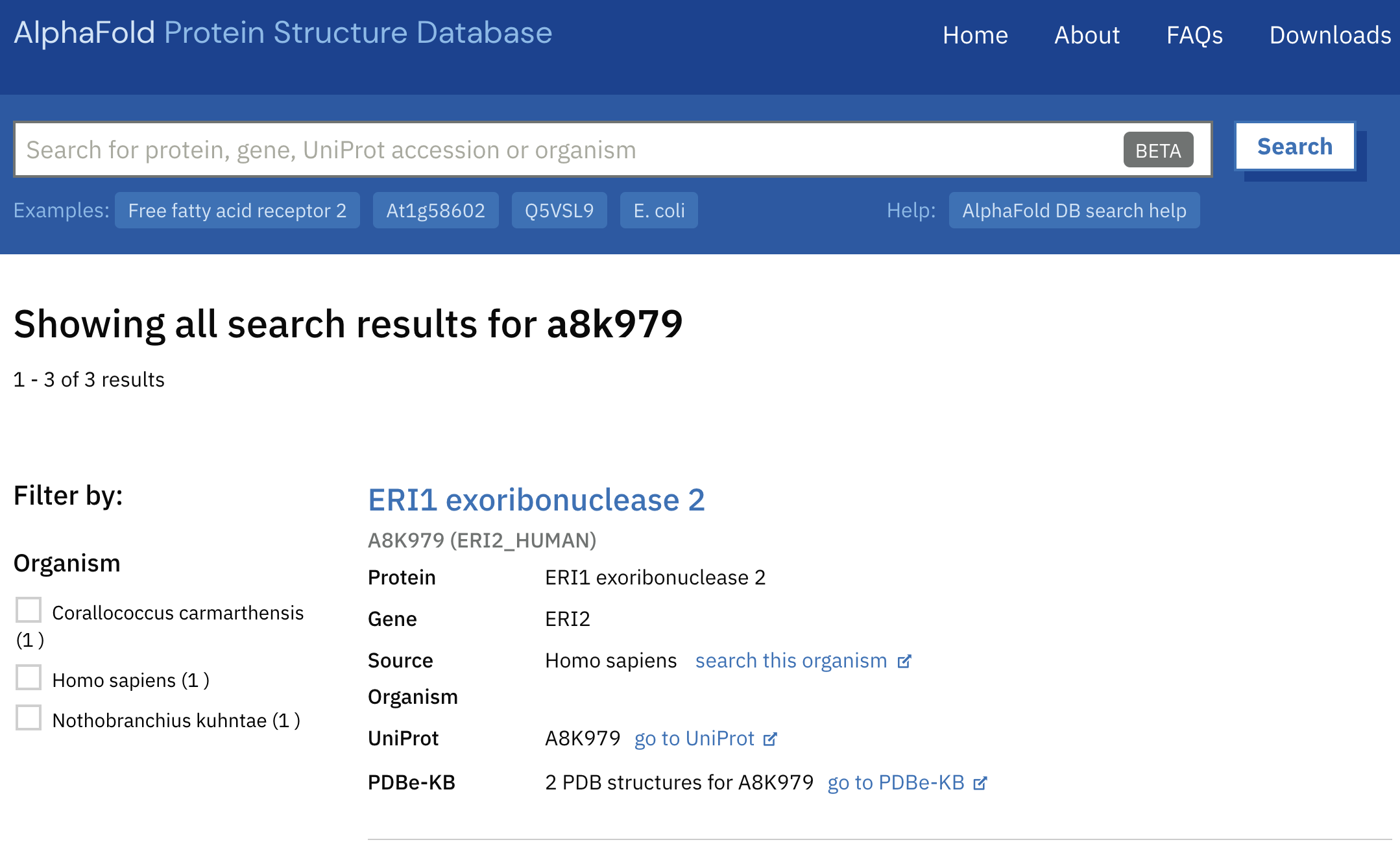
2. The database is searchable by protein name, gene, organism, and UniProt id. We'll search with a UniProt id. Enter a8k979 into the search bar and hit search.
3. The top result should be a human ERI1 exoribonuclease 2. Check the information in the search result. Note that this prediction has solved experimental PDB structures for reference, such as 7n8v encompassing residues 30-243. You will not always be so lucky!
4. Now click on the "ERI1 exoribonuclease 2" link to access the prediction. From this page, download the predicted structure by clicking "PDB file" next to Download. Scroll down to explore the prediction in the 3D interactive Mol* viewer. The structure is color-coded by pLDDT, a measure of prediction certainty, and shows a dark-blue confident region surrounded by long loops of orange low confidence.

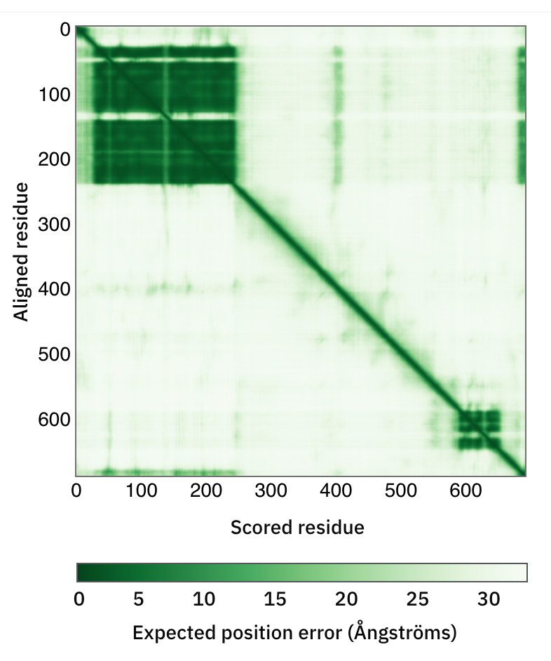
5. As in the image here, there is also a green “PAE” matrix that shows how confident the predicted relationships are between different parts of the sequence. Residues 34-242 with a strong off-diagonal square of relationships match the 7n8v template in this case, but parts without templates are also often predicted confidently and accurately.
6. Once you have downloaded the predicted structure, you can validate it with MolProbity. Go to http://molprobity.biochem.duke.edu, and instead of using the fetch function as before, use the "Choose File" button to select the alphafold PDB file you downloaded. Then hit "Upload >" to upload the file to the MolProbity server. "Add hydrogens", this time without flips (the prediction has no flip errors), and continue. Go to "Analyze all-atom contacts and geometry", accept all the defaults except “Suggest/report …” near the bottom, and run. It should take less than 2 minutes; if you get bored, take a look at the Ramachandran pdf, which, as we’ll see later, is quite strange.
7. Once the analysis has completed, note how the summary chart shows almost no clashes and no bond-length outliers, but almost everything else is terrible. To understand what this means, continue to the main page, scroll down to the Popular downloads section, and download (with a right-click) the multi.html under charts, the pdb file with H’s under coordinates, and the multi.kin, the cbetadev.kin and the rama.kin under kinemages. Then logout of MolProbity and delete your files.

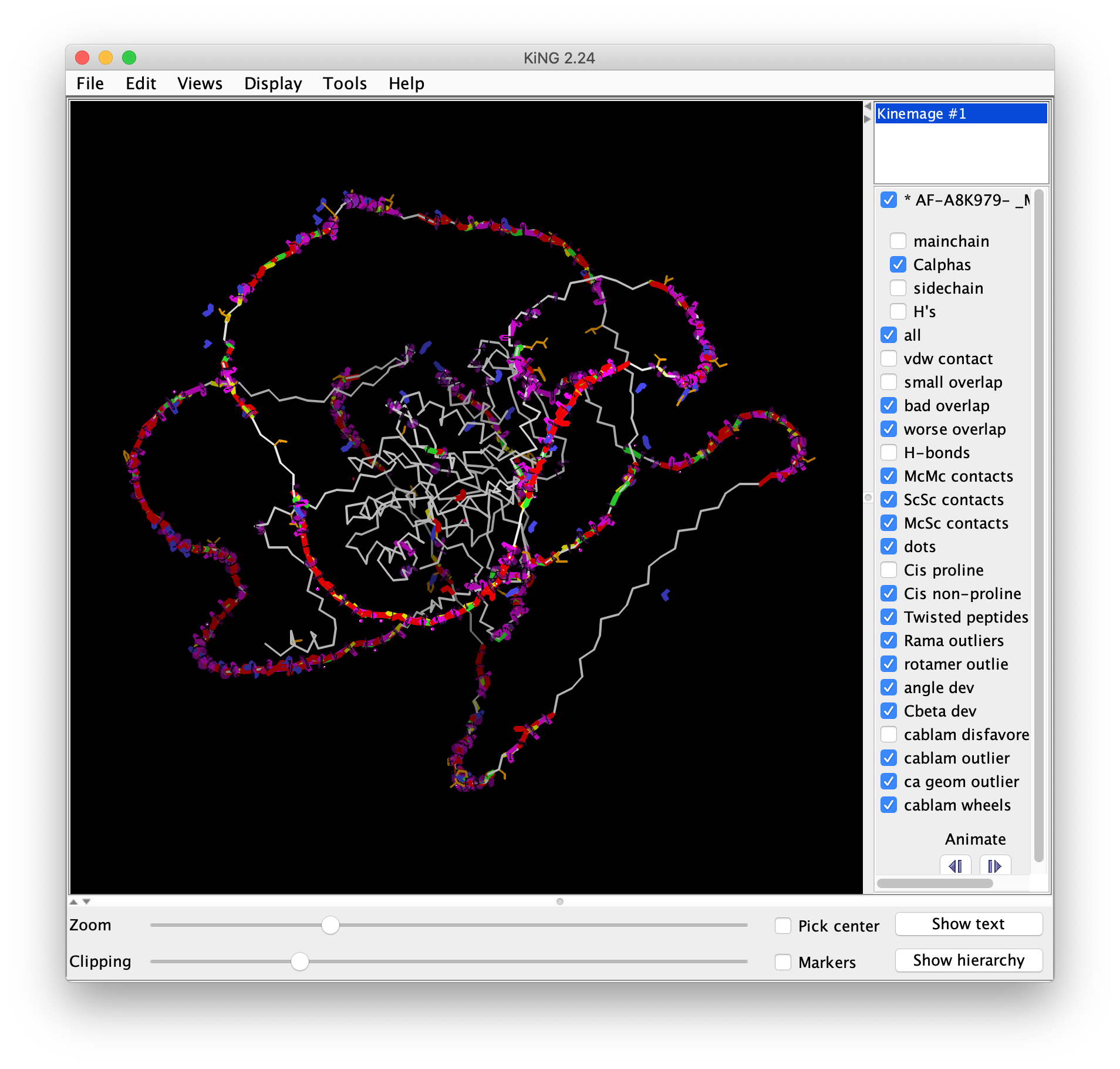
8. Open the multi.kin.gz file in KiNG. Note how the well-packed core of the protein has very few outliers, while the unmodelled "barbed-wire" regions where AlphaFold was unable to make a prediction contains all sorts of issues. This is an excellent reminder about why it is critical to look at either predicted or experimental structures to pinpoint the location of the errors, and to not just rely on global scores. It's completely possible that in an overall poor structure, your region of interest is modelled well, and conversely, in an overall good structure, your region of interest is modelled poorly.
9. Open the rama.kin file in KiNG and turn off the "Outlier Lbls" (labels) button. Notice that essentially all the outliers are in a band near +120° in psi. Animate through all 6 Ramachandran types to see how each behaves. The prolines are especially startling, because the ring closure normally constrains the phi dihedral close to -90°. It happens that the only backbone dihedral that is set for an isolated amino-acid-residue (as in the starting “residue gas” of the AlphaFold protocol) is the psi dihedral defined by N-Ca-C-N (but also set by N-Ca-C-O). Apparently the starting conformation AlphaFold uses is close to +120°, and when it has no information to make an actual prediction, that value is only tweaked a little when each one is translated to join barbed-wire residues in sequence order. That protocol gives extremely bad protein conformations. Let’s now look at that on the 3D structure.
10. If you didn't close the multi-kin earlier, you can switch back to it in KiNG by clicking in the kinemage list in the top right corner, and go back to the startup view. Otherwise, reopen the multi-kin. Starting at the bottom of the button panel, turn off each outlier type one at a time, to appreciate how many examples of how many types of outliers are ubiquitous in the barbed wire regions. Then turn them all back on again. Note, however, that there are stretches of the open loops with no outliers. In "Edit" > "Find point", type 548 in the search box and hit search to center in the longest of those stretches. Turn on mainchain and sidechain and turn off Calphas. Zoom in and move around a bit to appreciate that the sidechains and CO groups have an average 3-fold arrangement along this extended strand. There are 5 prolines in the 20 residues, and AlphaFold here lined up the residues in poly-proline II conformation which happens to have a psi value around +120° to +150° to match the psi of its original gas of individual residues, but a phi value of -60° to -90°, which happens to be a legal region of the Ramachandran plot. Move locally to Pro 536, just before this poly-Pro section. Turn off all 3 CaBLAM-related buttons. As well as being a Ramachandran outlier, the Pro ring has a very large twist, enabled at the expense of twisting the preceding peptide omega angle to an impossible 90°.
11. Close KiNG and open the multi html chart in a web browser. Just scroll down quickly and notice the great contrast between quiet parts of the sequence, where the prediction is very good, versus sections of barbed wire where nearly every residue has multiple outliers. There are almost no clashes or Cbeta deviations, and no bond-length outliers (columns 4, 7, & 9), but many residues have 5 outliers in Ramachandran, rotamer, CaBLAM, bond angle, and cis/twisted peptides. Close the chart window and go to Part 2: Rebuilding in KiNG.

http://kinemage.biochem.duke.edu/teaching/csh/

Jane & Dave Richardson