Patterson Function and Maps

This section needs a lot of work to bring in use with fiber diffraction and SAXS.

This is the heart of SAXS analysis, though in that field the various formulations to describe regions of particular interest are named by developers, rather than go under the general name of the person who (as I heard tell by Bert Warren) first realized the meaning of the plot of measured intensity as a function of angle from the incident beam direction.

In the special case of crystallography - a possible method for locating atom positions
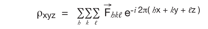
We can experimentally measure the intensity (I, or | F |²) of each spot in the diffraction pattern; but we do not know the phase of each F, so we cannot calculate the electron density map:

However, in order to make the best use of what information we do have we can calculate a special Fourier transform of the intensities: Note, magnitude of F is √I, but if calculate from F the complex number, multiply F with its complex conjugate.

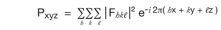
A plot of this function is called a Patterson map, and it has a peak for each vector between a pair of atoms in the crystal The size of each peak is the product of the number of electrons in each atom of that pair. (The Patterson function is usually expressed in terms of u,v,w, instead of x,y,z because it shows separations between atoms rather than real positions in space.) A sample simple structure and its Patterson map are shown on the next page.

In very simple cases one can reason backward from the Patterson map and discover the atom positions. Also, if there are a few heavy atoms that dominate the Patterson map then their positions can be determined and used to help solve the rest of the structure. With dominant heavy atom(s):
   |F_T| ∼ |F_H| and |φ_T| ∼ |φ_H|
Patterson map using |F_T|² (measured) ∼ Patterson map with |F_H|²

So in cases with just a few such dominant atoms, one locates the heavy atoms, calculates φ_H ∼ φ_T , calculates an approximation to the electron density map using those phases. That map will hopefully show at least some of the lighter atoms, which are used to get a better approximation to the phase for an improved electron density map which may show a few more atoms, etc., etc.

This method is used very frequently in small-molecule crystallography, but it is hopeless for proteins, where no atom could be big enough to dominate all those thousands of C,N, and O.

The trick for proteins is to do two experiments: One is as above with crystals of the Native Protein, and another with crystals of the Protein molecules containing a few places with Heavy Atom Isomorphous Replacements, i.e. where certain atoms or groups of atoms are replaced isomorphously by atoms with very different numbers of electrons. Most conveniently is to replace an atom in protein by a chemically compatible very heavy atom. Also works to replace solvent atoms with a specifically bound heavy atom or group with a heavy atom.

Measure diffraction from two crystals to get experimentally |F_PH| and |F_P|

where exactly F_PH = F_P + F_H (vectors with amplitude and phase),
but approximately: |F_PH| ∼ |F_P| + |F_H|
so solve the Patterson Map of relatively simple structure of the Heavy Atom replacement alone from
|F_H| ∼ |F_PH| - |F_P|
Using this to get phases for F_P is explained below in the section "Phasing: Isomorphous"
where we discover that we need yet a third set of experimental measurements to break the ambiguity left from the first two.

Patterson map from simple structure of 3 atoms

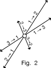
Figure 1 shows a single unit cell (repeating unit) of a simple 3-atom crystal structure, with all the vectors between pairs of atoms drawn in.

Figure 2 shows these vectors as starting from a common origin. The Patterson map has a peak at the end of each vector, plus an origin peak.

Any vector between atoms in different unit cells, as in the dotted arrow of Figure 3, is just the unit cell translation plus one of the vectors we already plotted.

Thus if we repeat the same pattern of peaks at each corner of the unit cell, as in Figure 4, we include all vectors between atoms.

Figure 5 shows what this same Patterson map would look like when plotted in the customary way as a contour map.

The challenge now is recognizing that this Patterson Map pattern might be from 3 atoms, and on that basis making a model of 3 atoms placed in the unit cell that would have produced the observed Pattern Map pattern.

Download:    PS-6-Patterson.pdf(140KB)  Problem set for this section