
Having looked at the characteristics of individual structural features and some of their local combinations, we are now in a position to sort out and classify the major structural patterns, or "folds," that make up entire proteins. This classification will build on earlier work by Rossmann (e.g., ), Richardson (), and Levitt and Chothia (), but will attempt to combine and extend those systems, as well as including the newer structures now available.
[In 2006, the major resources for classification of protein structures are SCOP (scop.mrc-lmb.cam.ac.uk/scop/) (Murzin, 1995) and CATH (www.cathdb.info/latest/index.html) (Orengo, 1997) which use major categories similar to the ones here: a lowest “family” level from sequence homology, and distinct versions of “fold”-based categories in between. Both are organized by domains. Further notes on the many new types of folds seen since 1981 will be found in the later sections.]
The most useful level at which to categorize protein structures is the domain, since there are many cases of multiple-domain proteins in which each separate domain resembles other entire smaller proteins. We have separated proteins into domains on the basis of whether the pieces could be expected to be stable as independent units or are analogous to other complete structures (see Section II,I for a fuller explanation). Clearly demonstrated homologous families such as trypsin, chymotrypsin, elastase, and the S. griseus proteases, or the cytochromes c, c2, c550, c551, and C555, are treated as single examples. There are between 90 and 105 different domains represented in the current sampling of known protein structures, depending on how one counts the cases of similar domain structures within a given protein. In the schematic drawings of Figs. 72-86 such domains are illustrated separately only if they are at least as different as the range of variation common within the close homology families (and, of course, if suitable coordinates or stereos were available). The domains within each protein are distinguished by numbers in sequence order (e.g., papain dl and papain d2), except for the immunoglobulins for which we use the standard terminology (VL, CH1, etc.) for constant and variable domains.
Structural categories are assigned primarily on the basis of the type and organization of secondary-structure elements, the topology of their connections, and the number of major layers of backbone structure that are present. Since proteins fold to form a protected hydrophobic core of side chains on the interior, the simplest type of stable protein structure consists of polypeptide backbone wrapped more or less uniformly around the outside of a single hydrophobic core. We will describe such a structure as "two layer," because a line from the solvent through the center of the protein and back out again would pass through two principal layers of backbone structure (see Fig. 71a). Over half of the known domain structures have two layers. About a third of the structures have three layers of backbone and two hydrophobic cores; the commonest such type has a central β sheet layer flanked by two helical layers (see Fig. 71b). There are three known four-layer domains (e.g., Fig. 71c) and one five-layer. Isolated loops that curl over the outside are not considered to form a distinct layer. Although there are some ambiguous cases (especially in the very small structures) they are less common than one might expect, presumably because the requirements for rapid folding rule out much tangling or recrossing of the backbone.
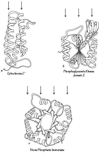
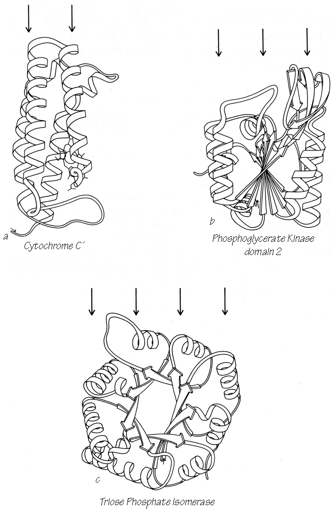
FIG. 71. Examples of protein domains with different numbers of layers of backbone structure: (a) two-layer cytochrome c'; (b) three-layer phosphoglycerate kinase domain 2; (c) four-layer triosephosphate isomerase. The arrows above each drawing point to the backbone layers.
The approximately 100 distinctly different domains fall into four broad categories, each of which has several subgroupings. The four broad categories are (I) antiparallel α; (II) parallel α/β; (III) antiparallel β; (IV) small SS-rich or metal-rich. The major determinant in assigning a domain to one of these categories is not just the percentage of a given secondary structure, but whether that type of secondary structure forms the central core and whether its interactions could be the dominant stabilizing ones. The two β categories are the most populous, with 30 to 35 members each; there are about 20 α-helical domains and a dozen of the small proteins. The overall classification scheme is summarized in Section III,A,2. An alphabetical index of the proteins is given in Section III,A,4, with domain assignments, structure subcategories, and literature references.
Obviously this classification is not the only plausible way to categorize protein structures. Indeed, for some of the individual cases there are other descriptions which would be preferable because they emphasize possible relationships to functionally similar proteins. However, the motivation here has been to achieve the most satisfactory compromise for all the structures: to fit as many examples into as few groupings as possible, while retaining enough detail to provide meaningful descriptions. Also, the prejudice has been in favor of grouping together domains whose entire structure is approximately the same rather than cases in which a relatively small portion of both structures is more exactly similar.
In order to illustrate this taxonomic system and to facilitate contrasts and comparisons among the structures, schematic backbone drawings have been made of most of the known structures. The drawings are grouped together by categories in Section III,A,3. α-Carbon coordinates were displayed in stereo on Richard Feldmann's computer graphics system at NIH; a suitable view was chosen (consistent for each subcategory of structure), and plotter output was obtained at a consistent scale (approximately 20Å per inch on the final drawings as reproduced here). The schematic was drawn on top of the plotter output for accuracy, with continual reference to the stereo for the third dimension. Loops, and to some extent β strands, were smoothed for comprehensibility, and shifts of 1 or 2Å were sometimes necessary in order to avoid ambiguity at crossing points. A uniform set of graphical conventions was adopted (see Section III,A,3 for explanation) in which β strands are shown as arrows, helices as spiral ribbons, and nonrepetitive structure as ropes. Location and extent of β strands and helices are sometimes based on published descriptions and hydrogen-bonding diagrams, but often must be judged from the stereo view itself. Very short β interactions are shown as arrows when they form part of a larger sheet but may be left out if they are isolated. Foreshortening, overlaps, edge appearance, and relative size change are used to provide depth cues.